The third term has just passed, and I would like to continue my last post on the discussion of some asymptotic properties and geometric interpretations for unbiased estimators.
m-estimators
Before we introduce the influence functions, let’s first have a overview of m-estimators.
Suppose we have data $D_1,…,D_n$, iid from a distribution $pr(D_i | \theta)$. Consider a function of $D_i$ and $\theta$, $g(D_i, \theta)$, such that
\[\begin{align*} E_{\theta}(g(D,\theta) | \theta) = 0 \end{align*}\]Then the estimator $\hat{\theta}$ is defined as the solution of the empirical average:
\[\begin{align*} \frac{1}{n} \sum_{i=1}^n g(D_i, \hat{\theta}) = 0 \end{align*}\]Under certain regularity conditions, we can prove the consistency and asymptotic normality of $\hat{\theta}$.
Influence functions
By mean value theorem, we can derive the following expansion:
\[\begin{align*} & \sum_{i=1}^n g(D_i, \hat{\theta}) = 0 \\ & \sum_{i=1}^n g(D_i, \theta_0) + \sum_{i=1}^n \frac{\partial g(D_i,\theta^* )}{\partial \theta} (\hat{\theta} - \theta_0) = 0 \end{align*}\]where $\theta^* $ is between $\theta_0$ and $\hat{\theta}$.
By the weak law of large numbers and regularity assumptions, we have
\[\begin{align*} \frac{1}{n} \sum_{i=1}^n \frac{\partial g(D_i,\theta^* )}{\partial \theta} \xrightarrow{p} E(\frac{\partial g(D,\theta^* )}{\partial \theta}) \end{align*}\]Then we have
\[\begin{align*} \sqrt{n} (\hat{\theta}-\theta) &= - [\frac{1}{n} \sum_{i=1}^n \frac{\partial g(D_i,\theta^* )}{\partial \theta} ]^{-1} \{ \frac{1}{\sqrt{n}} \sum_{i=1}^n g(D_i,\theta_0)\} \\ &= - [E(\frac{\partial g(D,\theta^* )}{\partial \theta}) ]^{-1} \{ \frac{1}{\sqrt{n}} \sum_{i=1}^n g(D_i,\theta_0)\}+o_p(1) \end{align*}\]Therefore, we can define the influence function as
\[\begin{align*} \phi(D_i) = - [E(\frac{\partial g(D,\theta^* )}{\partial \theta}) ]^{-1} g(D_i,\theta_0) \end{align*}\]It has the following property:
\[\begin{align*} \sqrt{n} (\hat{\theta}-\theta) = \frac{1}{\sqrt{n}} \sum_{i=1}^n \phi(D_i) + o_p(1) \end{align*}\]where $E(\phi(D))= 0$.
Geometric Interpretation
Now we are going to discuss about the geometry of influence functions for parametric models. Suppose the parameter $\theta$ can be represented as $(\beta^T,\eta^T)^T$, where $\beta$ is the parameter of interest with dimension $q$, $\eta$ is the nuisance parameter with dimension $r$, thus $\theta$ has dimension $p=q+r$.
Similar to the last post, we consider the Hilbert space of all $q$-dim random variables D with mean zero and finite variance, and inner product is defined as $<u,v>= E(u^T v)$. Then we define the tangent space spanned by the score vector $S_{\theta}(D,\theta_0)$:
\[\begin{align*} \Gamma = \{ A S_{\theta}(D,\theta_0) \ \text{for all matrices} \ A: q \times p \} \end{align*}\]The nuisance tangent is :
\[\begin{align*} \Gamma = \{ A S_{\eta}(D,\theta_0) \ \text{for all matrices} \ A: q \times r \} \end{align*}\]Now we can have an important theorem:
All influence functions can be represented as the linear variety $\phi^* (D) + \Gamma^{\perp}$, where $\phi^* (D)$ is any influence function and $\Gamma^{\perp}$ is the space orthogonal to the tangent space.
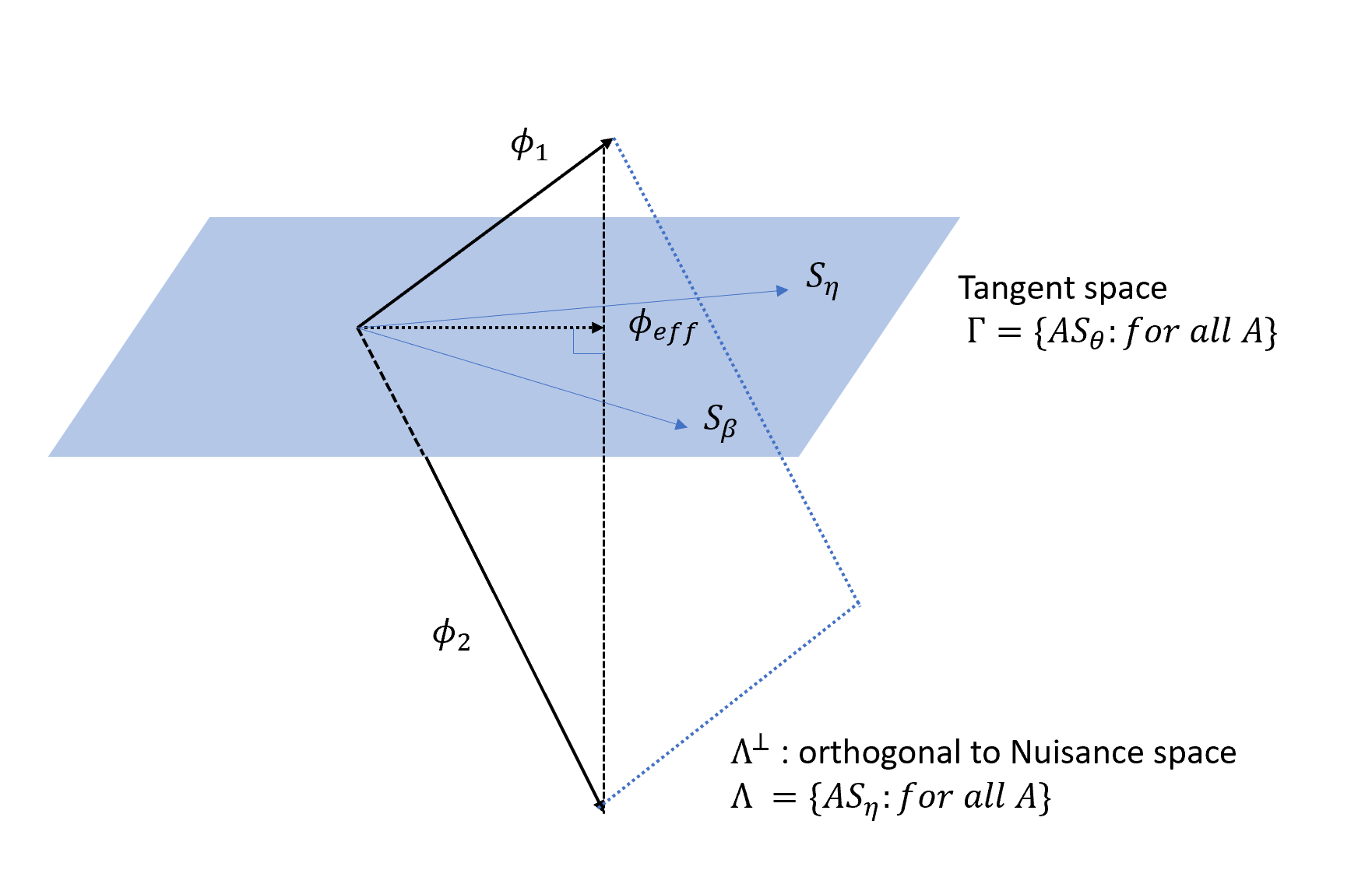
Then we can define the efficient function $\phi_{eff} (D)$, which has the smallest variance matrix. It is easy to prove that:
\[\begin{align*} \phi_{eff}(D) = \phi^* (D)- \Pi(\phi^* (D) | \Gamma^{\perp} ) = \Pi(\phi^* (D) | \Gamma) \end{align*}\]Reference
Lecture notes from Stats Theory, instructor: Prof.Constantine
Tsiatis, A. (2007). Semiparametric theory and missing data. Springer Science & Business Media.